In my last post, I wrote: in many robot policies, RL is gradually looking more and more like supervised learning.
This post dives into the specific method used by Pi0.6*: CFGRL. What makes it interesting is a new way of thinking about RL:
Policy improvement in RL can itself be rewritten as an inference problem under an optimality condition — and this inference problem can be implemented via classifier-free guidance at sampling time.
Once you think about it this way, the whole story starts to shift:
- Training doesn't necessarily require explicit, complex RL optimization;
- Training can remain a stable, generative process close to supervised learning;
- The actual "shift toward better actions" can happen at sampling / inference time.
In fact, several prior papers have explored similar ideas around test-time optimization, but this one is written with remarkable clarity, making the whole story easy to follow. So let me give a brief overview.
1. Starting from a Familiar Question: What Is RL Really Trying to Do?
If we set aside the implementation details — Bellman backup, TD targets, Actor-Critic — the core of RL is actually quite simple:
Given a reference policy, nudge it toward something better.
This reference policy could be:
- The behavior policy from a dataset,
- An imitation-learned policy,
- Or an already-trained generative policy.
A natural way to write the objective:
$$\max_\pi\; \mathbb{E}_{a\sim \pi(\cdot\mid s)}[Q(s,a)] -\alpha\,\mathrm{KL}\big(\pi(\cdot\mid s)\,\|\,\hat\pi(\cdot\mid s)\big)$$
Here $\hat\pi(a\mid s)$ is the reference policy. This objective expresses a simple balance:
- On one hand, we want actions with higher value $Q(s,a)$;
- On the other hand, we don't want the policy to drift too far from the reference distribution.
Solving this objective yields an elegant form:
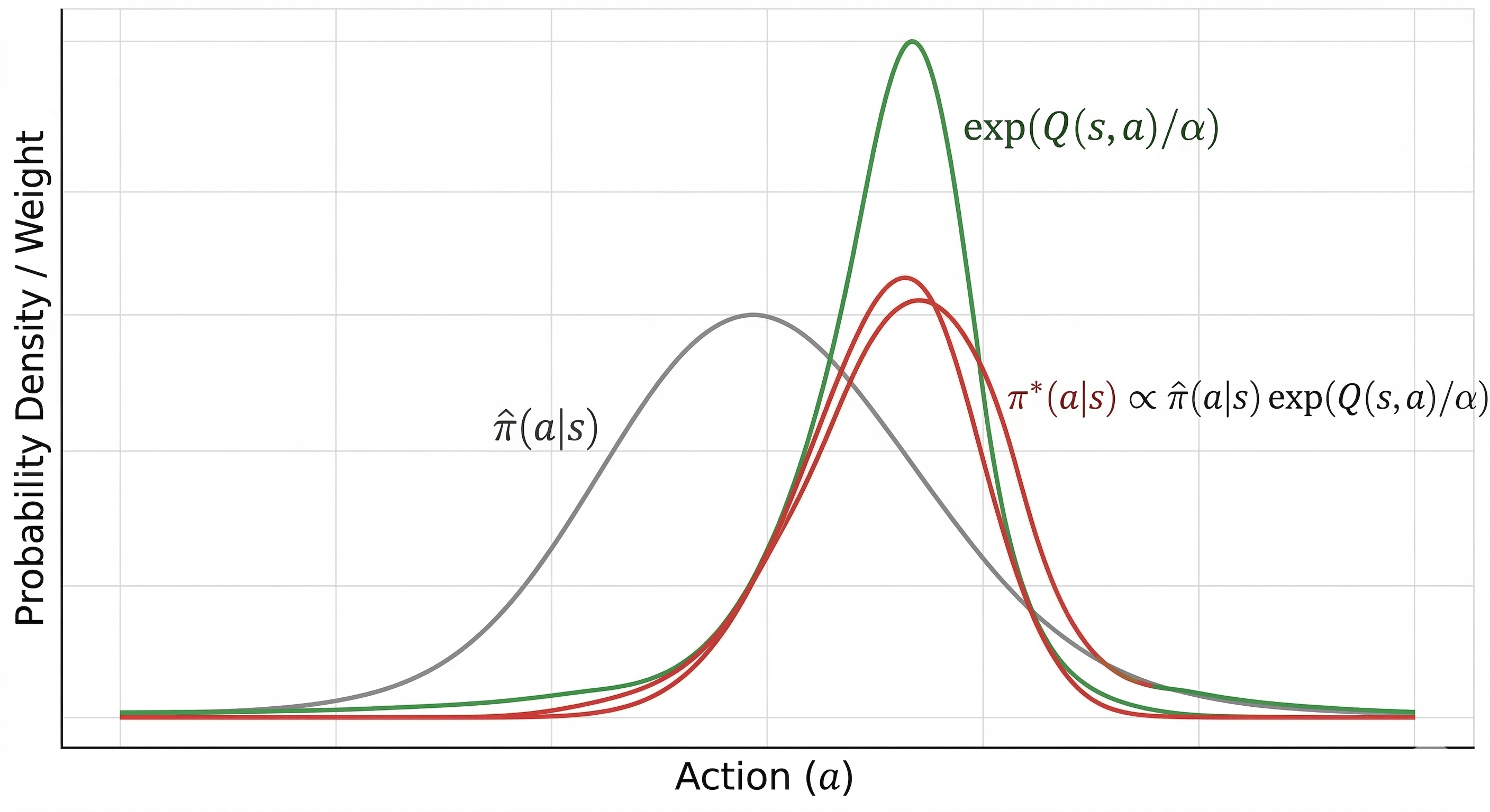
$$\pi^\star(a\mid s)\propto \hat\pi(a\mid s)\exp(Q(s,a)/\alpha)$$
This equation is arguably the most critical step in the entire paper.
It tells us that policy improvement doesn't necessarily mean learning an entirely "different" policy. More precisely, it's doing something gentler and more structured:
$$\text{improved policy} = \text{reference policy} \times \text{optimality weight}$$
In other words, the new policy isn't created from scratch — it reweights the original policy $\hat\pi$ by an "optimality factor." Actions with high $Q$ get amplified; actions with low $Q$ get suppressed.
This is important:
Policy improvement in RL can essentially be viewed as a product distribution (product policy).
2. Why Does the "Optimality Factor" Become an Inference Objective?
At this point, a natural question arises: $\exp(Q(s,a)/\alpha)$ — why can it be understood as an optimality term? And why is it related to "inference"?
This requires introducing a classic perspective: control as inference.
In traditional RL, we say:
Choose actions to maximize reward.
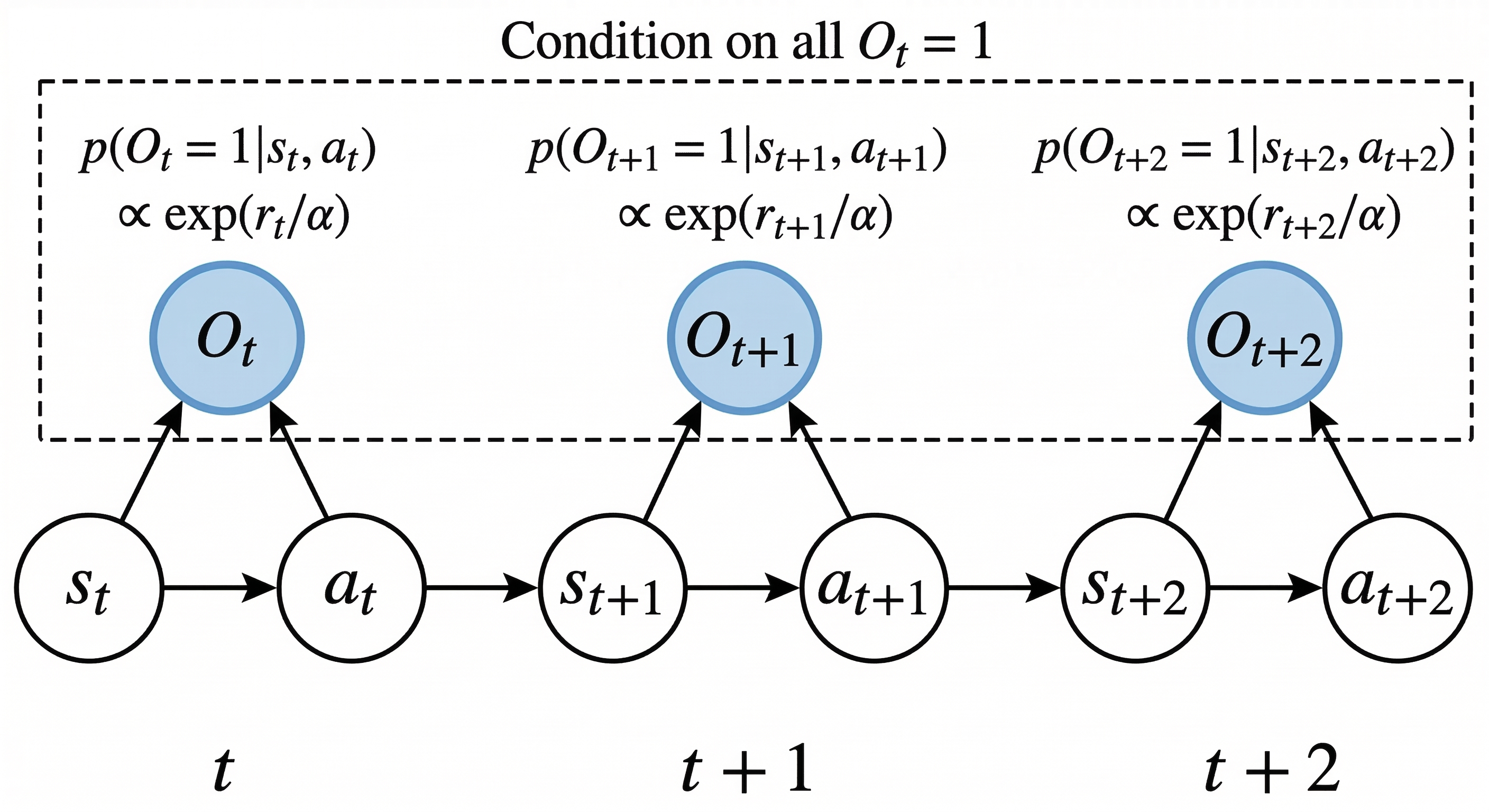
But in control-as-inference, we reframe it. We introduce a binary variable $O$:
$$O = 1 \quad \text{means the current state-action is optimal}$$
Then define a probabilistic model where high-reward actions are more likely to be deemed "optimal":
$$p(O=1\mid s,a)\propto \exp(r(s,a)/\alpha)$$
From this perspective, the control problem is no longer "directly optimize" but rather:
Given the observation that "this is optimal," infer which actions are more reasonable.
The original "max reward" problem is rewritten as a "posterior inference" problem. Levine's control-as-inference tutorial clearly formulates maximum-entropy RL in this probabilistic graphical model view, and SAC is built precisely on the maximum-entropy RL framework.
When we extend from one-step reward to the long-horizon setting, the optimality factor is no longer just $\exp(r/\alpha)$, but naturally corresponds to something like $\exp(Q/\alpha)$ — a long-horizon optimality weight. So the product policy from before:
$$\pi^\star(a\mid s)\propto \hat\pi(a\mid s)\exp(Q(s,a)/\alpha)$$
can be understood as:
The posterior distribution of the reference policy conditioned on optimality.
This step is crucial because it aligns two seemingly different things:
- On one side: policy improvement in RL;
- On the other: optimality-conditioned inference in probabilistic models.
And CFGRL's true contribution is built on this alignment.
3. A Second Look at CFG: What Is It Really Doing?
Now let's switch to the generative modeling side.
Classifier-Free Guidance (CFG) originally comes from conditional diffusion. The basic idea is very simple:
- Train a conditional model: $p(x\mid c)$
- Simultaneously train an unconditional model: $p(x)$
- At sampling time, instead of using only the conditional score, use:
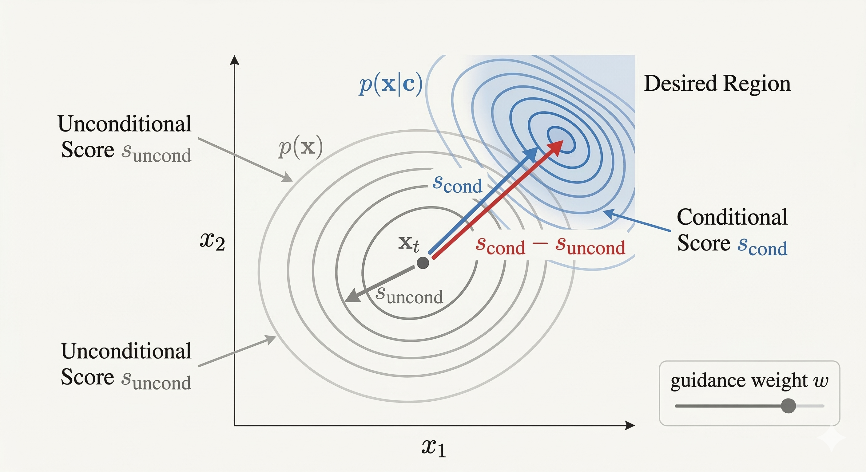
$$s_{\text{cfg}}(x) = s_{\text{uncond}}(x) + w\big(s_{\text{cond}}(x)-s_{\text{uncond}}(x)\big)$$
Here $w$ is the guidance weight. As $w$ increases, sampling shifts more strongly toward satisfying condition $c$. The key point of CFG: it doesn't need an additional classifier — it directly uses the difference between conditional and unconditional scores to get a "push toward the condition" signal.
From a generative modeling perspective alone, this is just a very useful sampling trick. But when you put it alongside the optimality inference framework, a striking structural similarity emerges:
- In RL, we want to start from the reference policy and nudge it toward "more optimal";
- In CFG, we're adding a "push toward the condition" guidance term on top of the base distribution.
This similarity is not a coincidence. CFGRL's core insight is: these two can actually be written as the same mathematical structure.
4. CFGRL's Key Step: Policy Improvement and CFG Are Isomorphic
We already have the product policy:
$$\pi(a\mid s)\propto \hat\pi(a\mid s)\,\mathcal{O}(s,a)$$
where $\mathcal{O}(s,a)$ is the optimality term — it can be a monotonic function of advantage or $Q$. CFGRL proves that as long as this optimality term is monotonic in advantage, it guarantees policy improvement; and increasing the guidance weight essentially strengthens the emphasis on optimality.
Now take the log-gradient in action space:
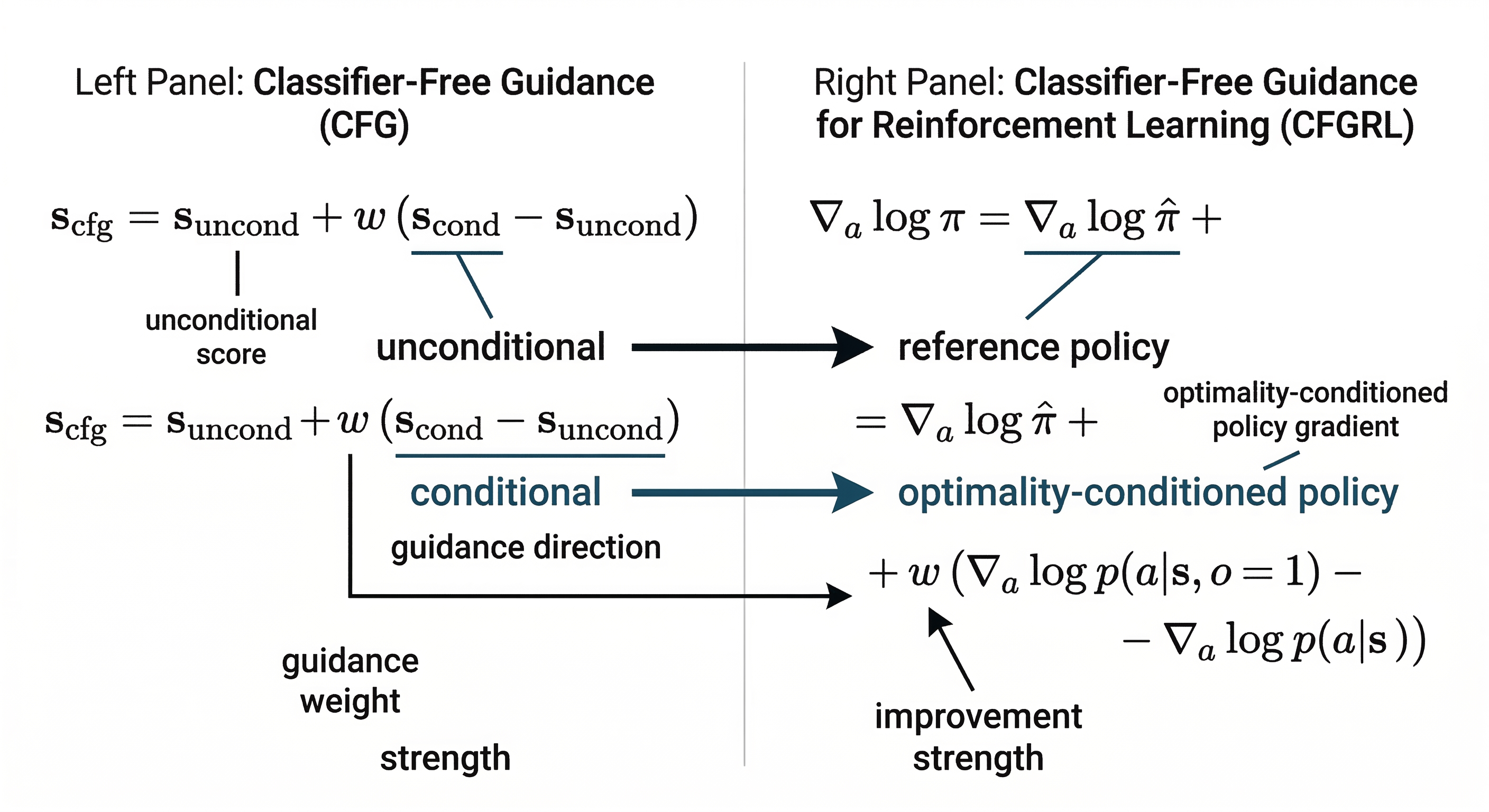
$$\nabla_a \log \pi(a\mid s) = \nabla_a \log \hat\pi(a\mid s) + \nabla_a \log \mathcal{O}(s,a)$$
This already looks very much like a "base score + guidance score" structure.
CFGRL introduces the optimality condition $o=1$, then uses Bayes' rule to get:
$$\nabla_a \log p(o=1\mid s,a) = \nabla_a \log p(a\mid s,o=1) - \nabla_a \log p(a\mid s)$$
That is, the optimality direction itself can be written as the difference of two scores:
- One is the optimality-conditioned policy score
- The other is the reference / unconditional policy score
So the full expression becomes:
$$s_{\text{guided}} = s_{\text{base}} + w\big(s_{\text{opt}}-s_{\text{base}}\big)$$
This is exactly the same form as CFG.
This is CFGRL's most central insight:
Classifier-free guidance doesn't just "look like" policy improvement — it structurally corresponds to a controllable policy improvement operator.
In other words, improvement in RL doesn't have to be done through parameter updates; it can also manifest as:
On a generative policy that has already learned the data distribution, use sampling-time guidance to push the output toward better regions.
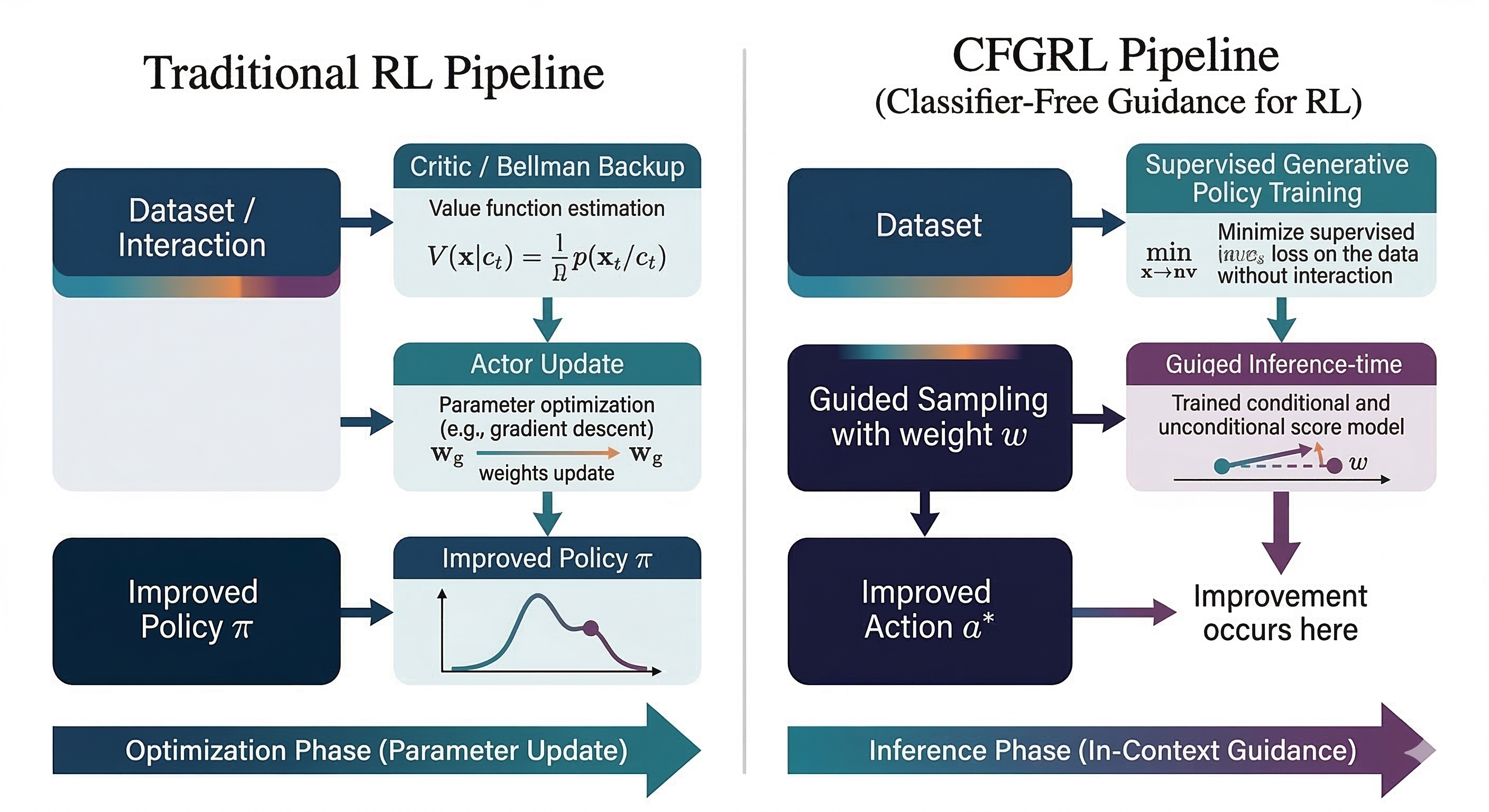
5. Why Does This Matter? It Moves "Improvement" from Training to Sampling
The default paradigm in traditional RL is:
- Do policy improvement during training;
- Only do forward inference at test time.
CFGRL offers another possibility:
- During training, maintain a more stable, supervised-learning-like generative modeling process;
- During sampling, complete policy improvement via guidance.
The most striking result in the CFGRL paper: as guidance weight increases, performance on offline RL tasks tends to steadily improve — and this improvement requires no model retraining. The authors summarize this as: train with supervised simplicity, but still achieve "beyond-data" improvement at inference time.
The implications are significant.
Many people have assumed that RL can surpass behavior cloning because it explicitly performs more complex optimization during training. CFGRL reminds us:
Perhaps "going beyond the data" doesn't have to come from a more complex training objective — it can also come from a smarter sampling operator.
This is a new perspective: shifting some of the "optimization burden" from the training phase to the inference phase.
6. Connecting Back: Why Is RL Looking More Like Supervised Learning?
If we place CFGRL back on the main thread from the previous post, it's pushing that trend one step further.
The previous post argued: with the development of offline RL, sequence modeling, diffusion policies, VLAs and other approaches, many methods that "belong to RL" are increasingly turning their core training process into:
- Conditional modeling,
- Weighted regression,
- Sequence prediction,
- Generative modeling.
In other words, training itself is looking more and more like supervised learning, while reward/value plays the role of reweighting, filtering, conditioning, or guidance.
CFGRL takes this logic to its natural conclusion:
- It no longer frames policy improvement primarily as Bellman backup;
- It first rewrites policy improvement as optimality inference;
- Then aligns this inference with CFG;
- Finally delegates the actual improvement to sampling-time guidance.
In this sense, CFGRL isn't departing from RL — it's extracting RL's most essential part — preference for better actions — and embedding it in a more stable, scalable, supervised-learning-like training paradigm.
7. Core Insights
Insight 1: Policy improvement can be written as a product policy
Policy improvement in RL doesn't have to start with Bellman backup. Under the KL-regularized view, it can be written as:
$$\pi^\star(a\mid s)\propto \hat\pi(a\mid s)\cdot \mathcal{O}(s,a)$$
i.e., "reference policy × optimality factor."
Insight 2: The optimality factor can be understood as an inference objective
Under the control-as-inference view, high reward / high value corresponds to "more likely to be optimal." Thus, policy improvement aligns with optimality-conditioned posterior inference.
Insight 3: Once in this form, RL becomes easier to cast as SL + Guided Sampling
This is why foundation models like π0.6 can first appear as supervised models, while subsequent improvement methods increasingly look like reward-aware conditioning, advantage-aware extraction, or sampling-time guidance applied on top of this supervised backbone.